Worked Examples
One of the best ways to learn XMDS2 is to see several illustrative examples. Here are a set of example scripts and explanations of the code, which will be a good way to get started. As an instructional aid, they are meant to be read sequentially, but the adventurous could try starting with one that looked like a simulation they wanted to run, and adapt for their own purposes.
The nonlinear Schrödinger equation (partial differential equation)
Kubo Oscillator (stochastic differential equations)
Fibre Noise (stochastic partial differential equation using parallel processing)
Integer Dimensions (integer dimensions)
Wigner Function (two dimensional PDE using parallel processing, passing arguments in at run time)
Finding the Ground State of a BEC (continuous renormalisation) (PDE with continual renormalisation - computed vectors, filters, breakpoints)
Finding the Ground State of a BEC again (Hermite-Gaussian basis)
Multi-component Schrödinger equation (combined integer and continuous dimensions with matrix multiplication, aliases)
All of these scripts are available in the included “examples” folder, along with more examples that demonstrate other tricks. Together, they provide starting points for a huge range of different simulations.
The nonlinear Schrödinger equation
This worked example will show a range of new features that can be used in an XMDS2 script, and we will also examine our first partial differential equation. We will take the one dimensional nonlinear Schrödinger equation, which is a common nonlinear wave equation. The equation describing this problem is:
where \(\phi\) is a complex-valued field, and \(\Gamma(\tau)\) is a \(\tau\)-dependent damping term. Let us look at an XMDS2 script that integrates this equation, and then examine it in detail.
<simulation xmds-version="2">
  <name>nlse</name>

  <author>Joe Hope</author>
  <description>
    The nonlinear Schrodinger equation in one dimension,
    which is a simple partial differential equation.
    We introduce several new features in this script.
  </description>

  <features>
      <benchmark />
      <bing />
      <fftw plan="patient" />
      <openmp />
      <auto_vectorise />
      <globals>
          <![CDATA[
          const double energy = 4;
          const double vel = 0.3;
          const double hwhm = 1.0;
          ]]>
       </globals>
     </features>

  <geometry>
      <propagation_dimension> xi </propagation_dimension>
      <transverse_dimensions>
        <dimension name="tau" lattice="128"  domain="(-6, 6)" />
      </transverse_dimensions>
   </geometry>

  <vector name="wavefunction" type="complex" dimensions="tau">
    <components> phi </components>
    <initialisation>
      <![CDATA[
      const double w0 = hwhm*sqrt(2/log(2));
      const double amp = sqrt(energy/w0/sqrt(M_PI/2));
      phi = amp*exp(-tau*tau/w0/w0)*exp(i*vel*tau);
      ]]>
    </initialisation>
  </vector>

  <vector name="dampingVector" type="real">
    <components> Gamma </components>
    <initialisation>
      <![CDATA[
      Gamma=1.0*(1-exp(-pow(tau*tau/4.0/4.0,10)));
      ]]>
    </initialisation>
  </vector>

  <sequence>
    <integrate algorithm="ARK45" interval="20.0" tolerance="1e-7">
      <samples>10 100 10</samples>
      <operators>
        <integration_vectors>wavefunction</integration_vectors>
        <operator kind="ex">
          <operator_names>Ltt</operator_names>
          <![CDATA[
            Ltt = -i*ktau*ktau*0.5;
          ]]>
        </operator>
        <![CDATA[
        dphi_dxi = Ltt[phi] - phi*Gamma + i*mod2(phi)*phi;
        ]]>
        <dependencies>dampingVector</dependencies>
      </operators>
    </integrate>
  </sequence>

  <output>
    <sampling_group basis="tau" initial_sample="yes">
      <moments>density</moments>
      <dependencies>wavefunction</dependencies>
      <![CDATA[
        density = mod2(phi);
      ]]>
    </sampling_group>

    <sampling_group basis="tau(0)" initial_sample="yes">
      <moments>normalisation</moments>
      <dependencies>wavefunction</dependencies>
      <![CDATA[
        normalisation = mod2(phi);
      ]]>
    </sampling_group>

    <sampling_group basis="ktau(32)" initial_sample="yes">
      <moments>densityK</moments>
      <dependencies>wavefunction</dependencies>
      <![CDATA[
        densityK = mod2(phi);
      ]]>
    </sampling_group>

  </output>
</simulation>
Let us examine the new items in the <features> element that we have demonstrated here. The existence of the <benchmark> element causes the simulation to be timed. The <bing> element causes the computer to make a sound upon the conclusion of the simulation. The <fftw> element is used to pass options to the FFTW libraries for fast Fourier transforms, which are needed to do spectral derivatives for the partial differential equation. Here we used the option plan=”patient”, which makes the simulation test carefully to find the fastest method for doing the FFTs. More information on possible choices can be found in the FFTW documentation.
Finally, we use two tags to make the simulation run faster. The <auto_vectorise> element switches on several loop optimisations that exist in later versions of the GCC compiler. The <openmp> element turns on threaded parallel processing using the OpenMP standard where possible. These options are not activated by default as they only exist on certain compilers. If your code compiles with them on, then they are recommended.
Let us examine the <geometry> element.
<geometry>
    <propagation_dimension> xi </propagation_dimension>
    <transverse_dimensions>
      <dimension name="tau" lattice="128"  domain="(-6, 6)" />
    </transverse_dimensions>
 </geometry>
This is the first example that includes a transverse dimension. We have only one dimension, and we have labelled it “tau”. It is a continuous dimension, but only defined on a grid containing 128 points (defined with the lattice variable), and on a domain from -6 to 6. The default is that transforms in continuous dimensions are fast Fourier transforms, which means that this dimension is effectively defined on a loop, and the “tau=-6” and “tau=6” positions are in fact the same. Other transforms are possible, as are discrete dimensions such as an integer-valued index, but we will leave these advanced possibilities to later examples.
Two vector elements have been defined in this simulation. One defines the complex-valued wavefunction “phi” that we wish to evolve. We define the transverse dimensions over which this vector is defined by the dimensions tag in the description. By default, it is defined over all of the transverse dimensions in the <geometry> element, so even though we have omitted this tag for the second vector, it also assumes that the vector is defined over all of tau.
The second vector element contains the component “Gamma” which is a function of the transverse variable tau, as specified in the equation of motion for the field. This second vector could have been avoided in two ways. First, the function could have been written explicitly in the integrate block where it is required, but calculating it once and then recalling it from memory is far more efficient. Second, it could have been included in the “wavefunction” vector as another component, but then it would have been unnecessarily complex-valued, it would have needed an explicit derivative in the equations of motion (presumably dGamma_dxi = 0;), and it would have been Fourier transformed whenever the phi component was transformed. So separating it as its own vector is far more efficient.
The <integrate> element for a partial differential equation has some new features:
<integrate algorithm="ARK45" interval="20.0" tolerance="1e-7">
  <samples>10 100 10</samples>
  <operators>
    <integration_vectors>wavefunction</integration_vectors>
    <operator kind="ex">
      <operator_names>Ltt</operator_names>
      <![CDATA[
        Ltt = -i*ktau*ktau*0.5;
      ]]>
    </operator>
    <![CDATA[
    dphi_dxi = Ltt[phi] - phi*Gamma + i*mod2(phi)*phi;
    ]]>
    <dependencies>dampingVector</dependencies>
  </operators>
</integrate>
There are some trivial changes from the tutorial script, such as the fact that we are using the ARK45 algorithm rather than ARK89. Higher order algorithms are often better, but not always. Also, since this script has multiple output groups, we have to specify how many times each of these output groups are sampled in the <samples> element, so there are three numbers there. Besides the vectors that are to be integrated, we also specify that we want to use the vector “dampingVector” during this integration. This is achieved by including the <dependencies> element inside the <operators> element.
The equation of motion as written in the CDATA block looks almost identical to our desired equation of motion, except for the term based on the second derivative, which introduces an important new concept. Inside the <operators> element, we can define any number of operators. Operators are used to define functions in the transformed space of each dimension, which in this case is Fourier space. The derivative of a function is equivalent to multiplying by \(i*k\) in Fourier space, so the \(\frac{i}{2}\frac{\partial^2 \phi}{\partial \tau^2}\) term in our equation of motion is equivalent to multiplying by \(-\frac{i}{2}k_\tau^2\) in Fourier space. In this example we define “Ltt” as an operator of exactly that form, and in the equation of motion it is applied to the field “phi”.
Operators can be explicit (kind="ex") or in the interaction picture (kind="ip"). The interaction picture can be more efficient, but it restricts the possible syntax of the equation of motion. Safe utilisation of interaction picture operators will be described later, but for now let us emphasise that explicit operators should be used unless the user is clear what they are doing. That said, XMDS2 will generate an error if the user tries to use interaction picture operators incorrectly. The constant="yes" option in the operator block means that the operator is not a function of the propagation dimension “xi”, and therefore only needs to be calculated once at the start of the simulation.
The output of a partial differential equation offers more possibilities than an ordinary differential equation, and we examine some in this example.
For vectors with transverse dimensions, we can sample functions of the vectors on the full lattice or a subset of the points. In the <sampling_group> element, we must add a string called “basis” that determines the space in which each transverse dimension is to be sampled, optionally followed by the number of points to be sampled in parentheses. If the number of points is not specified, it will default to a complete sampling of all points in that dimension. If a non-zero number of points is specified, it must be a factor of the lattice size for that dimension.
<sampling_group basis="tau" initial_sample="yes">
  <moments>density</moments>
  <dependencies>wavefunction</dependencies>
  <![CDATA[
    density = mod2(phi);
  ]]>
</sampling_group>
The first output group samples the mod square of the vector “phi” over the full lattice of 128 points.
If the lattice parameter is set to zero points, then the corresponding dimension is integrated.
<sampling_group basis="tau(0)" initial_sample="yes">
  <moments>normalisation</moments>
  <dependencies>wavefunction</dependencies>
  <![CDATA[
    normalisation = mod2(phi);
  ]]>
</sampling_group>
This second output group samples the normalisation of the wavefunction \(\int d\tau |\phi(\tau)|^2\) over the domain of \(\tau\). This output requires only a single real number per sample, so in the integrate element we have chosen to sample it many more times than the vectors themselves.
Finally, functions of the vectors can be sampled with their dimensions in Fourier space.
<sampling_group basis="ktau(32)" initial_sample="yes">
  <moments>densityK</moments>
  <dependencies>wavefunction</dependencies>
  <![CDATA[
    densityK = mod2(phi);
  ]]>
</sampling_group>
The final output group above samples the mod square of the Fourier-space wavefunction phi on a sample of 32 points.
Kubo Oscillator
This example demonstrates the integration of a stochastic differential equation. We examine the Kubo oscillator, which is a complex variable whose phase is evolving according to a Wiener noise. In a suitable rotating frame, the equation of motion for the variable is
where \(\eta(t)\) is the Wiener differential, and we interpret this as a Stratonovich equation. In other common notation, this is sometimes written:
Most algorithms employed by XMDS require the equations to be input in the Stratonovich form. Ito differential equations can always be transformed into Stratonovich equations, and in this case the difference is equivalent to the choice of rotating frame. This equation is solved by the following XMDS2 script:
<simulation xmds-version="2">
  <name>kubo</name>
  <author>Graham Dennis and Joe Hope</author>
  <description>
    Example Kubo oscillator simulation
  </description>

  <geometry>
    <propagation_dimension> t </propagation_dimension>
  </geometry>

  <driver name="multi-path" paths="10000" />

  <features>
    <error_check />
    <benchmark />
  </features>

  <noise_vector name="drivingNoise" dimensions="" kind="wiener" type="real" method="dsfmt" seed="314 159 276">
    <components>eta</components>
  </noise_vector>

  <vector name="main" type="complex">
    <components> z </components>
    <initialisation>
      <![CDATA[
        z = 1.0;
      ]]>
    </initialisation>
  </vector>

  <sequence>
    <integrate algorithm="SI" interval="10" steps="1000">
      <samples>100</samples>
      <operators>
        <integration_vectors>main</integration_vectors>
        <dependencies>drivingNoise</dependencies>
        <![CDATA[
          dz_dt = i*z*eta;
        ]]>
      </operators>
    </integrate>
  </sequence>

  <output>
    <sampling_group initial_sample="yes">
      <moments>zR zI</moments>
      <dependencies>main</dependencies>
      <![CDATA[
        zR = z.Re();
        zI = z.Im();
      ]]>
    </sampling_group>
  </output>
</simulation>
The first new item in this script is the <driver> element. This element enables us to change top level management of the simulation. Without this element, XMDS2 will integrate the stochastic equation as described. With this element and the option name="multi-path", it will integrate it multiple times, using different random numbers each time. The output will then contain the mean values and standard errors of your output variables. The number of integrations included in the averages is set with the paths variable.
In the <features> element we have included the <error_check> element. This performs the integration first with the specified number of steps (or with the specified tolerance), and then with twice the number of steps (or equivalently reduced tolerance). The output then includes the difference between the output variables on the coarse and the fine grids as the ‘error’ in the output variables. This error is particularly useful for stochastic integrations, where algorithms with adaptive step-sizes are less safe, so the number of integration steps must be user-specified.
We define the stochastic elements in a simulation with the <noise_vector> element.
<noise_vector name="drivingNoise" dimensions="" kind="wiener" type="real" method="dsfmt" seed="314 159 276">
 <components>eta</components>
</noise_vector>
This defines a vector that is used like any other, but it will be randomly generated with particular statistics and characteristics rather than initialised. The name, dimensions and type tags are defined just as for normal vectors. The names of the components are also defined in the same way. The noise is defined as a Wiener noise here (kind = "wiener"), which is a zero-mean Gaussian random noise with an average variance equal to the discretisation volume (here it is just the step size in the propagation dimension, as it is not defined over transverse dimensions). Other noise types are possible, including uniform and Poissonian noises, but we will not describe them in detail here.
We may also define a noise method to choose a non-default pseudo random number generator, and a seed for the random number generator. Using a seed can be very useful when debugging the behaviour of a simulation, and many compilers have pseudo-random number generators that are superior to the default option (posix).
The integrate block is using the semi-implicit algorithm (algorithm="SI"), which is a good default choice for stochastic problems, even though it is only second order convergent for deterministic equations. More will be said about algorithm choice later, but for now we should note that adaptive algorithms based on Runge-Kutta methods are not guaranteed to converge safely for stochastic equations. This can be particularly deceptive as they often succeed, particularly for almost any problem for which there is a known analytic solution.
We include elements from the noise vector in the equation of motion just as we do for any other vector. The default SI and Runge-Kutta algorithms converge to the Stratonovich integral. Ito stochastic equations can be converted to Stratonovich form and vice versa.
Executing the generated program ‘kubo’ gives slightly different output due to the “multi-path” driver.
$ ./kubo
Beginning full step integration ...
Starting path 1
Starting path 2

... many lines omitted ...

Starting path 9999
Starting path 10000
Beginning half step integration ...
Starting path 1
Starting path 2

... many lines omitted ...

Starting path 9999
Starting path 10000
Generating output for kubo
Maximum step error in moment group 1 was 4.942549e-04
Time elapsed for simulation is: 2.71 seconds
The maximum step error in each moment group is given in absolute terms. This is the largest difference between the full step integration and the half step integration. While a single path might be very stochastic:
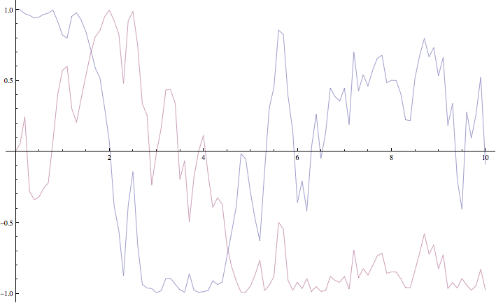
The mean value of the real and imaginary components of the z variable for a single path of the simulation.
The average over multiple paths can be increasingly smooth.
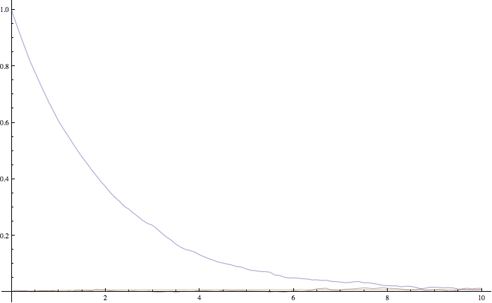
The mean and standard error of the z variable averaged over 10000 paths, as given by this simulation. It agrees within the standard error with the expected result of \(\exp(-t/2)\).
Fibre Noise
This simulation is a stochastic partial differential equation, in which a one-dimensional damped field is subject to a complex noise. This script can be found in examples/fibre.xmds.
where the noise terms \(\eta_j(x,t)\) are Wiener differentials and the equation is interpreted as a Stratonovich differential equation. On a finite grid, these increments have variance \(\frac{1}{\Delta x \Delta t}\).
<simulation xmds-version="2">
  <name>fibre</name>
  <author>Joe Hope and Graham Dennis</author>
  <description>
    Example fibre noise simulation
  </description>

  <geometry>
    <propagation_dimension> t </propagation_dimension>
    <transverse_dimensions>
      <dimension name="x" lattice="64"  domain="(-5, 5)" />
    </transverse_dimensions>
  </geometry>

  <driver name="mpi-multi-path" paths="8" />

  <features>
    <auto_vectorise />
    <benchmark />
    <error_check />
    <globals>
      <![CDATA[
      const real ggamma = 1.0;
      const real beta = sqrt(M_PI*ggamma/10.0);
      ]]>
    </globals>
  </features>

  <noise_vector name="drivingNoise" dimensions="x" kind="wiener" type="complex" method="dsfmt" seed="314 159 276">
    <components>Eta</components>
  </noise_vector>

  <vector name="main" initial_basis="x" type="complex">
    <components>phi</components>
    <initialisation>
      <![CDATA[
        phi = 0.0;
      ]]>
    </initialisation>
  </vector>

  <sequence>
    <integrate algorithm="SI" iterations="3" interval="2.5" steps="200000">
      <samples>50</samples>
      <operators>
        <operator kind="ex">
          <operator_names>L</operator_names>
          <![CDATA[
            L = -i*kx*kx;
          ]]>
        </operator>
        <dependencies>drivingNoise</dependencies>
        <integration_vectors>main</integration_vectors>
        <![CDATA[
          dphi_dt = L[phi] - ggamma*phi + beta*Eta;
        ]]>
      </operators>
    </integrate>
  </sequence>

  <output>
    <sampling_group basis="kx" initial_sample="yes">
      <moments>pow_dens</moments>
      <dependencies>main</dependencies>
      <![CDATA[
        pow_dens = mod2(phi);
      ]]>
    </sampling_group>
  </output>
</simulation>
Note that the noise vector used in this example is complex-valued, and has the argument dimensions="x" to define it as a field of delta-correlated noises along the x-dimension.
This simulation demonstrates the ease with which XMDS2 can be used in a parallel processing environment. Instead of using the stochastic driver “multi-path”, we simply replace it with “mpi-multi-path”. This instructs XMDS2 to write a parallel version of the program based on the widespread MPI standard. This protocol allows multiple processors or clusters of computers to work simultaneously on the same problem. Free open source libraries implementing this standard can be installed on a linux machine, and come standard on Mac OS X. They are also common on many supercomputer architectures. Parallel processing can also be used with deterministic problems to great effect, as discussed in the later example Wigner Function.
Executing this program is slightly different with the MPI option. The details can change between MPI implementations, but as an example:
$xmds2 fibre.xmds
xmds2 version 2.1 "Happy Mollusc" (r2543)
Copyright 2000-2012 Graham Dennis, Joseph Hope, Mattias Johnsson
                    and the xmds team
Generating source code...
... done
Compiling simulation...
... done. Type './fibre' to run.
Note that different compile options (and potentially a different compiler) are used by XMDS2, but this is transparent to the user. MPI simulations will have to be run using syntax that will depend on the MPI implementation. Here we show the version based on the popular open source Open-MPI implementation.
$ mpirun -np 4 ./fibre
Found enlightenment... (Importing wisdom)
Planning for x <---> kx transform... done.
Beginning full step integration ...
Rank[0]: Starting path 1
Rank[1]: Starting path 2
Rank[2]: Starting path 3
Rank[3]: Starting path 4
Rank[3]: Starting path 8
Rank[0]: Starting path 5
Rank[1]: Starting path 6
Rank[2]: Starting path 7
Rank[3]: Starting path 4
Beginning half step integration ...
Rank[0]: Starting path 1
Rank[2]: Starting path 3
Rank[1]: Starting path 2
Rank[3]: Starting path 8
Rank[0]: Starting path 5
Rank[2]: Starting path 7
Rank[1]: Starting path 6
Generating output for fibre
Maximum step error in moment group 1 was 4.893437e-04
Time elapsed for simulation is: 20.99 seconds
In this example we used four processors. The different processors are labelled by their “Rank”, starting at zero. Because the processors are working independently, the output from the different processors can come in a randomised order. In the end, however, the .xsil and data files are constructed identically to the single processor outputs.
The analytic solution to the stochastic averages of this equation is given by
where \(L_x\) is the length of the x domain. We see that a single integration of these equations is quite chaotic:
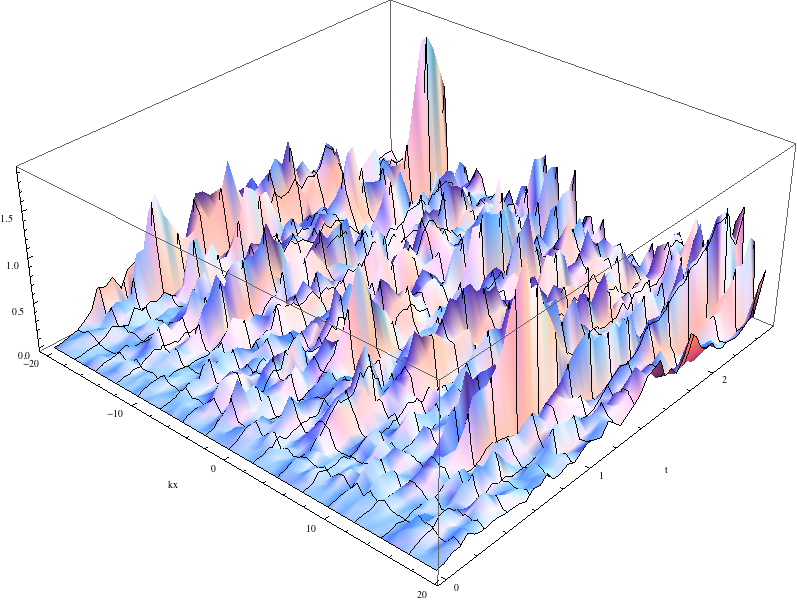
The momentum space density of the field as a function of time for a single path realisation.
while an average of 1024 paths (change paths="8" to paths="1024" in the <driver> element) converges nicely to the analytic solution:
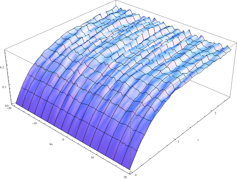
The momentum space density of the field as a function of time for an average of 1024 paths.
Integer Dimensions
This example shows how to handle systems with integer-valued transverse dimensions. We will integrate the following set of equations
where \(x_j\) are complex-valued variables defined on a ring, such that \(j\in \{0,j_{max}\}\) and the \(x_{j_{max}+1}\) variable is identified with the variable \(x_{0}\), and the variable \(x_{-1}\) is identified with the variable \(x_{j_{max}}\).
<simulation xmds-version="2">
  <name>integer_dimensions</name>
  <author>Graham Dennis</author>
  <description>
    XMDS2 script to test integer dimensions.
  </description>

  <features>
    <benchmark />
    <error_check />
    <bing />
    <diagnostics /> <!-- This will make sure that all nonlocal accesses of dimensions are safe -->
  </features>

  <geometry>
    <propagation_dimension> t </propagation_dimension>
    <transverse_dimensions>
      <dimension name="j" type="integer" lattice="5" domain="(0,4)" />
    </transverse_dimensions>
  </geometry>

  <vector name="main" type="complex">
    <components> x </components>
    <initialisation>
      <![CDATA[
      x = 1.0e-3;
      x(j => 0) = 1.0;
      ]]>
    </initialisation>
  </vector>

  <sequence>
    <integrate algorithm="ARK45" interval="60" steps="25000" tolerance="1.0e-9">
      <samples>1000</samples>
      <operators>
        <integration_vectors>main</integration_vectors>
        <![CDATA[
        long j_minus_one = (j-1) % _lattice_j;
        if (j_minus_one < 0)
          j_minus_one += _lattice_j;
        long j_plus_one  = (j+1) % _lattice_j;
        dx_dt(j => j) = x(j => j)*(x(j => j_minus_one) - x(j => j_plus_one));
        ]]>
      </operators>
    </integrate>
  </sequence>

  <output>
    <sampling_group basis="j" initial_sample="yes">
      <moments>xR</moments>
      <dependencies>main</dependencies>
      <![CDATA[
        xR = x.Re();
      ]]>
    </sampling_group>
  </output>
</simulation>
The first extra feature we have used in this script is the <diagnostics> element. It performs run-time checking that our generated code does not accidentally attempt to access a part of our vector that does not exist. Removing this tag will increase the speed of the simulation, but its presence helps catch coding errors.
The simulation defines a vector with a single transverse dimension labelled “j”, of type “integer” (“int” and “long” can also be used as synonyms for “integer”). In the absence of an explicit type, the dimension is assumed to be real-valued. The dimension has a “domain” argument as normal, defining the minimum and maximum values of the dimension’s range. The lattice element, if specified, is used as a check on the size of the domain, and will create an error if the two do not match.
Integer-valued dimensions can be called non-locally. Real-valued dimensions are typically coupled non-locally only through local operations in the transformed space of the dimension, but can be called non-locally in certain other situations as described in the reference. The syntax for calling integer dimensions non-locally can be seen in the initialisation CDATA block:
x = 1.0e-3;
x(j => 0) = 1.0;
where the syntax x(j => 0) is used to reference the variable \(x_0\) directly. We see a more elaborate example in the integrate CDATA block:
dx_dt(j => j) = x(j => j)*(x(j => j_minus_one) - x(j => j_plus_one));
where the vector “x” is called using locally defined variables. This syntax is chosen so that multiple dimensions can be addressed non-locally with minimal possibility for confusion.
Wigner Function
This example integrates the two-dimensional partial differential equation
with the added restriction that the derivative is forced to zero outside a certain radius. This extra condition helps maintain the long-term stability of the integration. The script can be found in examples/wigner_arguments_mpi.xmds under your XMDS2 installation directory.
<simulation xmds-version="2">
  <name>wigner</name>
  <author>Graham Dennis and Joe Hope</author>
  <description>
    Simulation of the Wigner function for an anharmonic oscillator with the initial state
    being a coherent state.
  </description>
  <features>
    <benchmark />
    <globals>
      <![CDATA[
        real Uint_hbar_on16;
      ]]>
    </globals>
    <arguments>
      <argument name="omega" type="real" default_value="0.0" />
      <argument name="alpha_0"     type="real" default_value="3.0" />
      <argument name="absorb"     type="real" default_value="8.0" />
      <argument name="width" type="real" default_value="0.3" />
      <argument name="Uint_hbar" type="real" default_value="1.0" />
      <![CDATA[
        /* derived constants */
        Uint_hbar_on16 = Uint_hbar/16.0;
      ]]>
    </arguments>
    <bing />
    <fftw plan="patient" />
    <openmp />
  </features>

  <driver name="distributed-mpi" />

  <geometry>
    <propagation_dimension> t </propagation_dimension>
    <transverse_dimensions>
      <dimension name="x" lattice="128"  domain="(-6, 6)" />
      <dimension name="y" lattice="128"  domain="(-6, 6)" />
    </transverse_dimensions>
  </geometry>

  <vector name="main" initial_basis="x y" type="complex">
    <components> W </components>
    <initialisation>
      <![CDATA[
        W = 2.0/M_PI * exp(-2.0*(y*y + (x-alpha_0)*(x-alpha_0)));
      ]]>
    </initialisation>
  </vector>

  <vector name="dampConstants" initial_basis="x y" type="real">
    <components>damping</components>
    <initialisation>
      <![CDATA[
      if (sqrt(x*x + y*y) > _max_x-width)
        damping = 0.0;
      else
        damping = 1.0;
      ]]>
    </initialisation>
  </vector>

  <sequence>
    <integrate algorithm="ARK89" tolerance="1e-7" interval="7.0e-4" steps="100000">
      <samples>50</samples>
      <operators>
        <operator kind="ex">
          <operator_names>Lx Ly Lxxx Lxxy Lxyy Lyyy</operator_names>
          <![CDATA[
            Lx = i*kx;
            Ly = i*ky;
            Lxxx = -i*kx*kx*kx;
            Lxxy = -i*kx*kx*ky;
            Lxyy = -i*kx*ky*ky;
            Lyyy = -i*ky*ky*ky;
          ]]>
        </operator>
        <integration_vectors>main</integration_vectors>
        <dependencies>dampConstants</dependencies>
        <![CDATA[
        real rotation = omega + Uint_hbar*(-1.0 + x*x + y*y);

        dW_dt = damping * ( rotation * (x*Ly[W] - y*Lx[W])
                    - Uint_hbar_on16*( x*(Lxxy[W] + Lyyy[W]) - y*(Lxyy[W] + Lxxx[W]) )
                );
        ]]>
      </operators>
    </integrate>
  </sequence>

  <output>
    <sampling_group basis="x y" initial_sample="yes">
      <moments>WR WI</moments>
      <dependencies>main</dependencies>
      <![CDATA[
        _SAMPLE_COMPLEX(W);
      ]]>
    </sampling_group>
  </output>
</simulation>
This example demonstrates two new features of XMDS2. The first is the use of parallel processing for a deterministic problem. The FFTW library only allows MPI processing of multidimensional vectors. For multidimensional simulations, the generated program can be parallelised simply by adding the name="distributed-mpi" argument to the <driver> element.
$ xmds2 wigner_argument_mpi.xmds
xmds2 version 2.1 "Happy Mollusc" (r2680)
Copyright 2000-2012 Graham Dennis, Joseph Hope, Mattias Johnsson
                    and the xmds team
Generating source code...
... done
Compiling simulation...
... done. Type './wigner' to run.
To use multiple processors, the final program is then called using the (implementation specific) MPI wrapper:
$ mpirun -np 2 ./wigner
Planning for (distributed x, y) <---> (distributed ky, kx) transform... done.
Planning for (distributed x, y) <---> (distributed ky, kx) transform... done.
Sampled field (for moment group #1) at t = 0.000000e+00
Current timestep: 5.908361e-06
Sampled field (for moment group #1) at t = 1.400000e-05
Current timestep: 4.543131e-06

...
The possible acceleration achievable when parallelising a given simulation depends on a great many things including available memory and cache. As a general rule, it will improve as the simulation size gets larger, but the easiest way to find out is to test. The optimum speed up is obviously proportional to the number of available processing cores.
The second new feature in this simulation is the <arguments> element in the <features> block. This is a way of specifying global variables with a given type that can then be input at run time. The variables are specified in a self explanatory way
<arguments>
  <argument name="omega" type="real" default_value="0.0" />
    ...
  <argument name="Uint_hbar" type="real" default_value="1.0" />
</arguments>
where the “default_value” is used as the valuable of the variable if no arguments are given. In the absence of the generating script, the program can document its options with the --help argument:
$ ./wigner --help
Usage: wigner --omega <real> --alpha_0 <real> --absorb <real> --width <real> --Uint_hbar <real>

Details:
Option              Type            Default value
-o,  --omega        real            0.0
-a,  --alpha_0      real            3.0
-b,  --absorb       real            8.0
-w,  --width        real            0.3
-U,  --Uint_hbar    real            1.0
We can change one or more of these variables’ values in the simulation by passing it at run time.
$ mpirun -np 2 ./wigner --omega 0.1 --alpha_0 2.5 --Uint_hbar 0
Found enlightenment... (Importing wisdom)
Planning for (distributed x, y) <---> (distributed ky, kx) transform... done.
Planning for (distributed x, y) <---> (distributed ky, kx) transform... done.
Sampled field (for moment group #1) at t = 0.000000e+00
Current timestep: 1.916945e-04

...
The values that were used for the variables, whether default or passed in, are stored in the output file (wigner.xsil).
<info>
Script compiled with XMDS2 version 2.1 "Happy Mollusc" (r2680)
See http://www.xmds.org for more information.

Variables that can be specified on the command line:
  Command line argument omega = 1.000000e-01
  Command line argument alpha_0 = 2.500000e+00
  Command line argument absorb = 8.000000e+00
  Command line argument width = 3.000000e-01
  Command line argument Uint_hbar = 0.000000e+00
</info>
Finally, note the shorthand used in the output group
<![CDATA[
  _SAMPLE_COMPLEX(W);
]]>
which is short for
<![CDATA[
  WR = W.Re();
  WI = W.Im();
]]>
Finding the Ground State of a BEC (continuous renormalisation)
This simulation solves another partial differential equation, but introduces several powerful new features in XMDS2. The nominal problem is the calculation of the lowest energy eigenstate of a non-linear Schrödinger equation:
which can be found by evolving the above equation in imaginary time while keeping the normalisation constant. This causes eigenstates to exponentially decay at the rate of their eigenvalue, so after a short time only the state with the lowest eigenvalue remains. The evolution equation is straightforward:
but we will need to use new XMDS2 features to manage the normalisation of the function \(\phi(y,t)\). The normalisation for a non-linear Schrödinger equation is given by \(\int dy |\phi(y,t)|^2 = N_{particles}\), where \(N_{particles}\) is the number of particles described by the wavefunction.
The code for this simulation can be found in examples/groundstate_workedexamples.xmds:
<simulation xmds-version="2">
  <name>groundstate</name>
  <author>Joe Hope</author>
  <description>
    Calculate the ground state of the non-linear Schrodinger equation in a harmonic magnetic trap.
    This is done by evolving it in imaginary time while re-normalising each timestep.
  </description>

  <features>
    <auto_vectorise />
    <benchmark />
    <bing />
    <fftw plan="exhaustive" />
    <globals>
      <![CDATA[
        const real Uint = 2.0;
        const real Nparticles = 5.0;
      ]]>
    </globals>
  </features>

  <geometry>
    <propagation_dimension> t </propagation_dimension>
    <transverse_dimensions>
      <dimension name="y" lattice="256"  domain="(-15.0, 15.0)" />
    </transverse_dimensions>
  </geometry>

  <vector name="potential" initial_basis="y" type="real">
    <components> V1 </components>
    <initialisation>
      <![CDATA[
        V1  = 0.5*y*y;
      ]]>
    </initialisation>
  </vector>

  <vector name="wavefunction" initial_basis="y" type="complex">
    <components> phi </components>
    <initialisation>
      <![CDATA[
        if (fabs(y) < 3.0) {
          phi = 1.0;
          // This will be automatically normalised later
        } else {
          phi = 0.0;
        }
            ]]>
    </initialisation>
  </vector>

  <computed_vector name="normalisation" dimensions="" type="real">
    <components> Ncalc </components>
    <evaluation>
      <dependencies basis="y">wavefunction</dependencies>
      <![CDATA[
        // Calculate the current normalisation of the wave function.
        Ncalc = mod2(phi);
      ]]>
    </evaluation>
  </computed_vector>

  <sequence>
      <filter>
        <![CDATA[
          printf("Hello world from a filter segment!\n");
        ]]>
      </filter>

    <filter>
        <dependencies>normalisation wavefunction</dependencies>
      <![CDATA[
        phi *= sqrt(Nparticles/Ncalc);
      ]]>
    </filter>

    <integrate algorithm="ARK45" interval="1.0" steps="4000" tolerance="1e-10">
      <samples>25 4000</samples>
      <filters where="step end">
        <filter>
          <dependencies>wavefunction normalisation</dependencies>
          <![CDATA[
            // Correct normalisation of the wavefunction
            phi *= sqrt(Nparticles/Ncalc);
          ]]>
        </filter>
      </filters>
      <operators>
        <operator kind="ip">
          <operator_names>T</operator_names>
          <![CDATA[
            T = -0.5*ky*ky;
          ]]>
        </operator>
        <integration_vectors>wavefunction</integration_vectors>
        <dependencies>potential</dependencies>
        <![CDATA[
          dphi_dt = T[phi] - (V1 + Uint*mod2(phi))*phi;
        ]]>
      </operators>
    </integrate>

    <breakpoint filename="groundstate_break.xsil">
      <dependencies basis="ky">wavefunction </dependencies>
    </breakpoint>

  </sequence>

  <output>
    <sampling_group basis="y" initial_sample="yes">
      <moments>norm_dens</moments>
      <dependencies>wavefunction normalisation</dependencies>
      <![CDATA[
        norm_dens = mod2(phi);
      ]]>
    </sampling_group>

    <sampling_group initial_sample="yes">
      <moments>norm</moments>
      <dependencies>normalisation</dependencies>
      <![CDATA[
        norm = Ncalc;
      ]]>
    </sampling_group>
  </output>
</simulation>
We have used the plan="exhaustive" option in the <fftw> element to ensure that the absolute fastest transform method is found. Because the FFTW package stores the results of its tests (by default in the ~/.xmds/wisdom directory), this option does not cause significant computational overhead, except perhaps on the very first run of a new program.
This simulation introduces the first example of a very powerful feature in XMDS2: the <computed_vector> element. This has syntax like any other vector, including possible dependencies on other vectors, and an ability to be used in any element that can use vectors. The difference is that, much like noise vectors, computed vectors are recalculated each time they are required. This means that a computed vector can never be used as an integration vector, as its values are not stored. However, computed vectors allow a simple and efficient method of describing complicated functions of other vectors. Computed vectors may depend on other computed vectors, allowing for spectral filtering and other advanced options. See for example, the Advanced Topics section on Convolutions and Fourier transforms.
The difference between a computed vector and a stored vector is emphasised by the replacement of the <initialisation> element with an <evaluation> element. Apart from the name, they have virtually identical purpose and syntax.
<computed_vector name="normalisation" dimensions="" type="real">
  <components> Ncalc </components>
  <evaluation>
    <dependencies basis="y">wavefunction</dependencies>
    <![CDATA[
      // Calculate the current normalisation of the wave function.
      Ncalc = mod2(phi);
    ]]>
  </evaluation>
</computed_vector>
Here, our computed vector has no transverse dimensions and depends on the components of “wavefunction”, so the extra transverse dimensions are integrated out. This code therefore integrates the square modulus of the field, and returns it in the variable “Ncalc”. This will be used below to renormalise the “phi” field. Before we examine that process, we have to introduce the <filter> element.
The <filter> element can be placed in the <sequence> element, or inside <integrate> elements as we will see next. Elements placed in the <sequence> element are executed in the order they are found in the .xmds file. Filter elements place the included CDATA block directly into the generated program at the designated position. If the element does not contain any dependencies, like in our first example, then the code is placed alone:
<filter>
  <![CDATA[
    printf("Hello world from a filter segment!\n");
  ]]>
</filter>
This filter block merely prints a string into the output when the generated program is run. If the <filter> element contains dependencies, then the variables defined in those vectors (or computed vectors, or noise vectors) will be available, and the CDATA block will be placed inside loops that run over all the transverse dimensions used by the included vectors. The second filter block in this example depends on both the “wavefunction” and “normalisation” vectors:
<filter>
    <dependencies>normalisation wavefunction</dependencies>
  <![CDATA[
    phi *= sqrt(Nparticles/Ncalc);
  ]]>
</filter>
Since this filter depends on a vector with the transverse dimension “y”, this filter will execute for each point in “y”. This code multiplies the value of the field “phi” by the factor required to produce a normalised function in the sense that \(\int dy |\phi(y,t)|^2 = N_{particles}\).
The next usage of a <filter> element in this program is inside the <integrate> element, where all filters are placed inside a <filters> element.
<filters where="step end">
  <filter>
    <dependencies>wavefunction normalisation</dependencies>
    <![CDATA[
      // Correct normalisation of the wavefunction
      phi *= sqrt(Nparticles/Ncalc);
    ]]>
  </filter>
</filters>
Filters placed in an integration block are applied each integration step. The “where” flag is used to determine whether the filter should be applied directly before or directly after each integration step. The default value for the where flag is where="step start", but in this case we chose “step end” to make sure that the final output was normalised after the last integration step.
At the end of the sequence element we introduce the <breakpoint> element. This serves two purposes. The first is a simple matter of convenience. Often when we manage our input and output from a simulation, we are interested solely in storing the exact state of our integration vectors. A breakpoint element does exactly that, storing the components of any vectors contained within, taking all the normal options of the <output> element but not requiring any <sampling_group> elements as that information is assumed.
<breakpoint filename="groundstate_break.xsil">
  <dependencies basis="ky">wavefunction</dependencies>
</breakpoint>
If the filename argument is omitted, the output filenames are numbered sequentially. Any given <breakpoint> element must only depend on vectors with identical dimensions.
This program begins with a very crude guess to the ground state, but it rapidly converges to the lowest eigenstate.
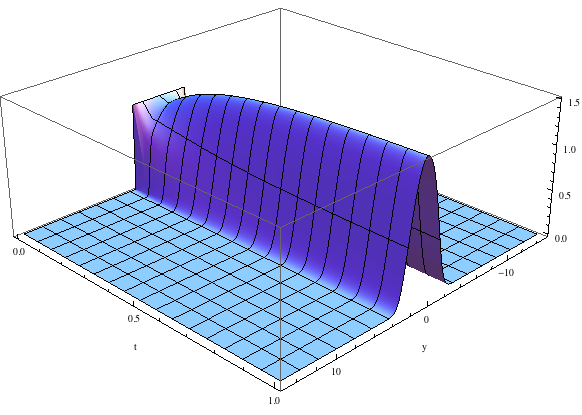
The shape of the ground state rapidly approaches the lowest eigenstate. For weak nonlinearities, it is nearly Gaussian.
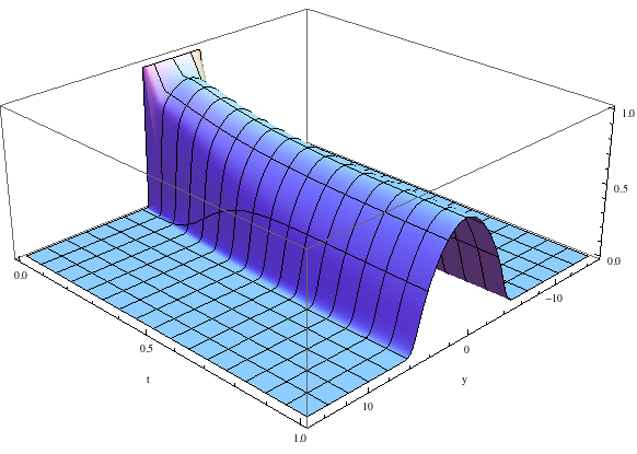
When the nonlinear term is larger (\(U=20\)), the ground state is wider and more parabolic.
Finding the Ground State of a BEC again
Here we repeat the same simulation as in the Finding the Ground State of a BEC (continuous renormalisation) example, using a different transform basis. While spectral methods are very effective, and Fourier transforms are typically very efficient due to the Fast Fourier transform algorithm, it is often desirable to describe nonlocal evolution in bases other than the Fourier basis. The previous calculation was the Schrödinger equation with a harmonic potential and a nonlinear term. The eigenstates of such a system are known analytically to be Gaussians multiplied by the Hermite polynomials.
where
where \(H_n(u)\) are the physicist’s version of the Hermite polynomials. Rather than describing the derivatives as diagonal terms in Fourier space, we therefore have the option of describing the entire \(-\frac{\hbar}{2 m}\frac{\partial^2}{\partial x^2} + \frac{1}{2}\omega^2 x^2\) term as a diagonal term in the Hermite-Gaussian basis. Here is an XMDS2 simulation that performs the integration in this basis. The following is a simplified version of the examples/hermitegauss_groundstate.xmds script.
<simulation xmds-version="2">
  <name>hermitegauss_groundstate</name>
  <author>Graham Dennis</author>
  <description>
    Solve for the groundstate of the Gross-Pitaevskii equation using the Hermite-Gauss basis.
  </description>

  <features>
    <benchmark />
    <bing />
    <validation kind="run-time" />
    <globals>
      <![CDATA[
        const real omegaz = 2*M_PI*20;
        const real omegarho = 2*M_PI*200;
        const real hbar = 1.05457148e-34;
        const real M = 1.409539200000000e-25;
        const real g = 9.8;
        const real scatteringLength = 5.57e-9;
        const real transverseLength = 1e-5;
        const real Uint = 4.0*M_PI*hbar*hbar*scatteringLength/M/transverseLength/transverseLength;
        const real Nparticles = 5.0e5;

        /* offset constants */
        const real EnergyOffset = 0.3*pow(pow(3.0*Nparticles/4*omegarho*Uint,2.0)*M/2.0,1/3.0); // 1D
      ]]>
    </globals>
  </features>

  <geometry>
    <propagation_dimension> t </propagation_dimension>
    <transverse_dimensions>
      <dimension name="x" lattice="100" length_scale="sqrt(hbar/(M*omegarho))" transform="hermite-gauss" />
    </transverse_dimensions>
  </geometry>

  <vector name="wavefunction" initial_basis="x" type="complex">
    <components> phi </components>
    <initialisation>
      <![CDATA[
      phi = sqrt(Nparticles) * pow(M*omegarho/(hbar*M_PI), 0.25) * exp(-0.5*(M*omegarho/hbar)*x*x);
      ]]>
    </initialisation>
  </vector>

  <computed_vector name="normalisation" dimensions="" type="real">
    <components> Ncalc </components>
    <evaluation>
      <dependencies basis="x">wavefunction</dependencies>
      <![CDATA[
        // Calculate the current normalisation of the wave function.
        Ncalc = mod2(phi);
      ]]>
    </evaluation>
  </computed_vector>

  <sequence>
    <integrate algorithm="ARK45" interval="1.0e-2" steps="4000"  tolerance="1e-10">
      <samples>100 100</samples>
      <filters>
        <filter>
          <dependencies>wavefunction normalisation</dependencies>
          <![CDATA[
            // Correct normalisation of the wavefunction
            phi *= sqrt(Nparticles/Ncalc);
          ]]>
        </filter>
      </filters>
      <operators>
        <operator kind="ip" type="real">
          <operator_names>L</operator_names>
          <![CDATA[
            L = EnergyOffset/hbar - (nx + 0.5)*omegarho;
          ]]>
        </operator>
        <integration_vectors>wavefunction</integration_vectors>
        <![CDATA[
          dphi_dt = L[phi] - Uint/hbar*mod2(phi)*phi;
        ]]>
      </operators>
    </integrate>

    <filter>
        <dependencies>normalisation wavefunction</dependencies>
      <![CDATA[
        phi *= sqrt(Nparticles/Ncalc);
      ]]>
    </filter>

    <breakpoint filename="hermitegauss_groundstate_break.xsil" format="ascii">
      <dependencies basis="nx">wavefunction</dependencies>
    </breakpoint>
  </sequence>

  <output>
    <sampling_group basis="x" initial_sample="yes">
      <moments>dens</moments>
      <dependencies>wavefunction</dependencies>
      <![CDATA[
        dens = mod2(phi);
      ]]>
    </sampling_group>
    <sampling_group basis="kx" initial_sample="yes">
      <moments>dens</moments>
      <dependencies>wavefunction</dependencies>
      <![CDATA[
        dens = mod2(phi);
      ]]>
    </sampling_group>
  </output>
</simulation>
The major difference in this simulation code, aside from the switch back from dimensionless units, is the new transverse dimension type in the <geometry> element.
<dimension name="x" lattice="100" length_scale="sqrt(hbar/(M*omegarho))" transform="hermite-gauss" />
We have explicitly defined the “transform” option, which by default expects the Fourier transform. The transform="hermite-gauss" option requires the ‘mpmath’ package installed, just as Fourier transforms require the FFTW package to be installed. The “lattice” option details the number of hermite-Gaussian eigenstates to include, and automatically starts from the zeroth order polynomial and increases. The number of hermite-Gaussian modes fully determines the irregular spatial grid up to an overall scale given by the length_scale parameter.
The length_scale="sqrt(hbar/(M*omegarho))" option requires a real number, but since this script defines it in terms of variables, XMDS2 is unable to verify that the resulting function is real-valued at the time of generating the code. XMDS2 will therefore fail to compile this program without the feature:
<validation kind="run-time" />
which disables many of these checks at the time of writing the C-code.
Multi-component Schrödinger equation
This example demonstrates a simple method for doing matrix calculations in XMDS2. We are solving the multi-component PDE
where the last term is more commonly written as a matrix multiplication. Writing this term out explicitly is feasible for a small number of components, but when the number of components becomes large, or perhaps \(V_{j k}\) should be precomputed for efficiency reasons, it is useful to be able to perform this sum over the integer dimensions automatically. This example show how this can be done naturally using a computed vector. The XMDS2 script is as follows:
<simulation xmds-version="2">
  <name>2DMSse</name>

  <author>Joe Hope</author>
  <description>
    Schroedinger equation for multiple internal states in two spatial dimensions.
  </description>

  <features>
      <benchmark />
      <bing />
      <fftw plan="patient" />
      <openmp />
      <auto_vectorise />
     </features>

  <geometry>
      <propagation_dimension> t </propagation_dimension>
      <transverse_dimensions>
          <dimension name="x" lattice="32"  domain="(-6, 6)" />
          <dimension name="y" lattice="32"  domain="(-6, 6)" />
          <dimension name="j" type="integer" lattice="2" domain="(0,1)" aliases="k"/>
      </transverse_dimensions>
   </geometry>

  <vector name="wavefunction" type="complex" dimensions="x y j">
    <components> phi </components>
    <initialisation>
      <![CDATA[
      phi = j*sqrt(2/sqrt(M_PI/2))*exp(-(x*x+y*y)/4)*exp(i*0.1*x);
      ]]>
    </initialisation>
  </vector>

  <vector name="spatialInteraction" type="real" dimensions="x y">
    <components> U </components>
    <initialisation>
      <![CDATA[
      U=exp(-(x*x+y*y)/4);
      ]]>
    </initialisation>
  </vector>

  <vector name="internalInteraction" type="real" dimensions="j k">
    <components> V </components>
    <initialisation>
      <![CDATA[
      V=3*(j*(1-k)+(1-j)*k);
      ]]>
    </initialisation>
  </vector>

  <computed_vector name="coupling" dimensions="x y j" type="complex">
    <components>
      VPhi
    </components>
    <evaluation>
      <dependencies basis="x y j k">internalInteraction wavefunction</dependencies>
      <![CDATA[
        // Calculate the current normalisation of the wave function.
        VPhi = V*phi(j => k);
      ]]>
    </evaluation>
  </computed_vector>

  <sequence>
    <integrate algorithm="ARK45" interval="2.0" tolerance="1e-7">
      <samples>20 100</samples>
      <operators>
        <integration_vectors>wavefunction</integration_vectors>
        <operator kind="ip" dimensions="x">
          <operator_names>Lx</operator_names>
          <![CDATA[
            Lx = -i*kx*kx*0.5;
          ]]>
        </operator>
        <operator kind="ip" dimensions="y">
          <operator_names>Ly</operator_names>
          <![CDATA[
            Ly = -i*ky*ky*0.5;
          ]]>
        </operator>
        <![CDATA[
        dphi_dt = Lx[phi] + Ly[phi] -i*U*VPhi;
        ]]>
        <dependencies>spatialInteraction coupling</dependencies>
      </operators>
    </integrate>
  </sequence>

  <output>
    <sampling_group basis="x y j" initial_sample="yes">
      <moments>density</moments>
      <dependencies>wavefunction</dependencies>
      <![CDATA[
        density = mod2(phi);
      ]]>
    </sampling_group>
    <sampling_group basis="x(0) y(0) j" initial_sample="yes">
      <moments>normalisation</moments>
      <dependencies>wavefunction</dependencies>
      <![CDATA[
        normalisation = mod2(phi);
      ]]>
    </sampling_group>
  </output>
</simulation>
The only truly new feature in this script is the “aliases” option on a dimension. The integer-valued dimension in this script indexes the components of the PDE (in this case only two). The \(V_{j k}\) term is required to be a square array of dimension of this number of components. If we wrote the k-index of \(V_{j k}\) using a separate <dimension> element, then we would not be enforcing the requirement that the matrix be square. Instead, we note that we will be using multiple ‘copies’ of the j-dimension by using the “aliases” tag.
<dimension name="j" type="integer" lattice="2" domain="(0,1)" aliases="k"/>
This means that we can use the index “k”, which will have exactly the same properties as the “j” index. This is used to define the “V” function in the “internalInteraction” vector. Now, just as we use a computed vector to perform an integration over our fields, we use a computed vector to calculate the sum.
<computed_vector name="coupling" dimensions="x y j" type="complex">
  <components>
    VPhi
  </components>
  <evaluation>
    <dependencies basis="x y j k">internalInteraction wavefunction</dependencies>
    <![CDATA[
      // Calculate the current normalisation of the wave function.
      VPhi = V*phi(j => k);
    ]]>
  </evaluation>
</computed_vector>
Since the output dimensions of the computed vector do not include a “k” index, this index is integrated. The volume element for this summation is the spacing between neighbouring values of “j”, and since this spacing is one, this integration is just a sum over k, as required.
This example also demonstrates an optimisation for the IP operators by separating the \(x\) and \(y\) parts of the operator (see Optimising with the Interaction Picture (IP) operator). This gives an approximately 30% speed improvement over the more straightforward implementation:
<operator kind="ip">
  <operator_names>L</operator_names>
  <![CDATA[
    L = -i*(kx*kx + ky*ky)*0.5;
  ]]>
</operator>
<![CDATA[
  dphi_dt = L[phi] - i*U*VPhi;
]]>
By this point, we have introduced most of the important features in XMDS2. More details on other transform options and rarely used features can be found in the Advanced Topics section.